Learnt Image Compression
ref: EE274-2023-lec16
Introduction
Image compression is about reducing the redundacy stored in an image.
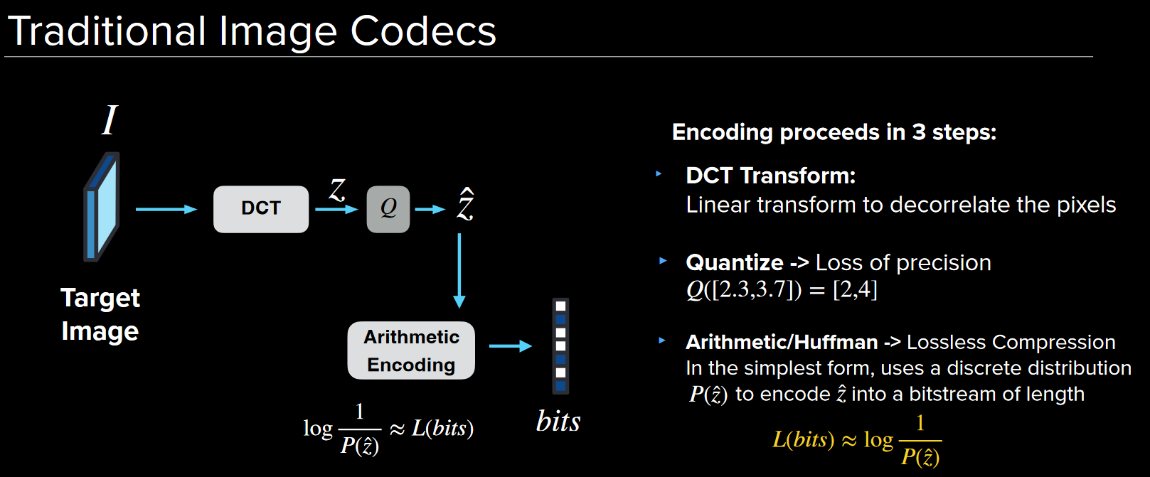
In traditional methods like JPEG, the image is converted and quantinized, followed by a lossess compression.
The color space transformation and DCT are linear operations, and its possible to do better with non-linear operations.
Also, there are tons of hand tuned parameters in JPEG, which can be learned by a neural network.
ML Review
ML is essentially using linear combinations and non-linear activation functions to approximate the relationship inside data.
The key to learn is to use gradient descent to update the weights and minimize the loss function, and backpropagation is the algorithm to calculate this.
After a forward pass, the parameter is at a known function composed of the loss function, the activation functions and the activation values, making the calculation of the gradient a direct process.
One requirement for the backpropagation to work is that all the functions in the process need to be differentiable.
Autoencoder
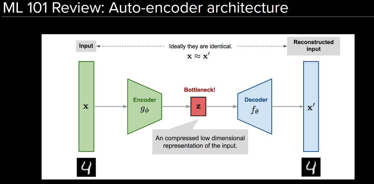
Autoencoder is an unsupervised learning algorithm that contains a bottle neck layer with small number of neurons, and the loss function is the difference between the input and the output.
This forces the network to learn the most important features of the input, and the bottleneck layer is the compressed representation of the input.
Learnt Image Compression
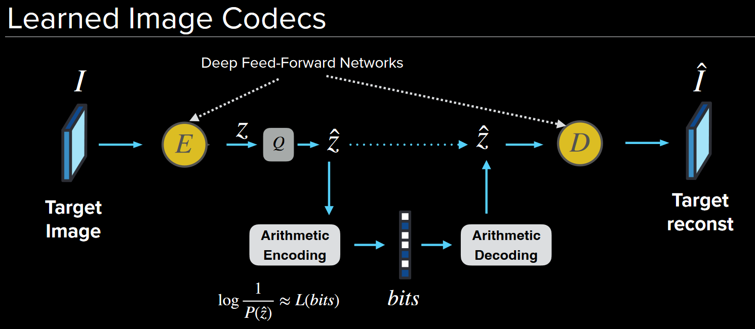
To design an end-to-end ML model for image compression, a direct approach is to replace the DCT/I-DCT transform with an autoencoder network:
In order to train this network, a loss function is needed to be deisgned.
Based on the Rate-Distorion theory, the loss function should be in the form of $L = R + \lambda D$, aiming to minimizing two terms and balancing the trade-off between them.
The rate term $R$ is the number of bits needed to represent the compressed image, and the distortion term $D$ is the difference between the input and the output.
The rate can be expressed as the entropy, which is calculated from the distribution of the compressed representation $-\log{P(\hat{z})}$
Therefore, the whole loss function can be expressed as:
$L = -\log P(\hat{z}) + \lambda d(I, \hat I)$
However, the discrete entropy is not differentiable. The solution is to approximate it using a continuous distribution(Variational AutoEncoder, VAE), like $\cal{N}(0, 1)$: $P(\hat{z}) = \text{CDF}(\hat{z} + 0.5) - \text{CDF}(\hat{z} - 0.5)$
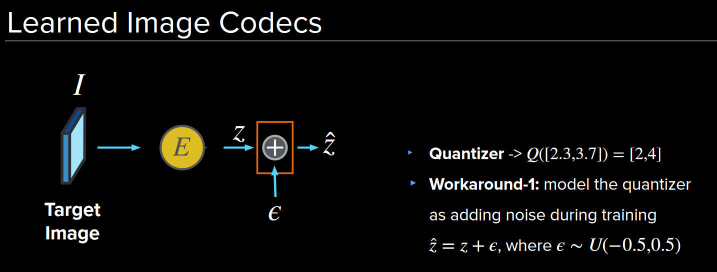
Another problem is the quantinizaiton process, which is also not differentiable. The workaroud is to view it as adding a constant noise to the compressed representation, which doen’t affect the gradient.
Hence, we have a trainable end-to-end ML model for image compression now.
Q&A
Q: How can the model calculate the gradient if the loss is calculated from an intermidiate layer?
A: When the loss is backpropagated to the relavant layer, the related gradient can be calculated directly from the loss function instead of the previous layer’s gradient.
Q: How can we ensure that the encoded representation is of the determined distribution?
A: As the approximated distribution’s entropy is minimized, the model will learn to generate the encoded representation that is close to the distribution.
